Business problem
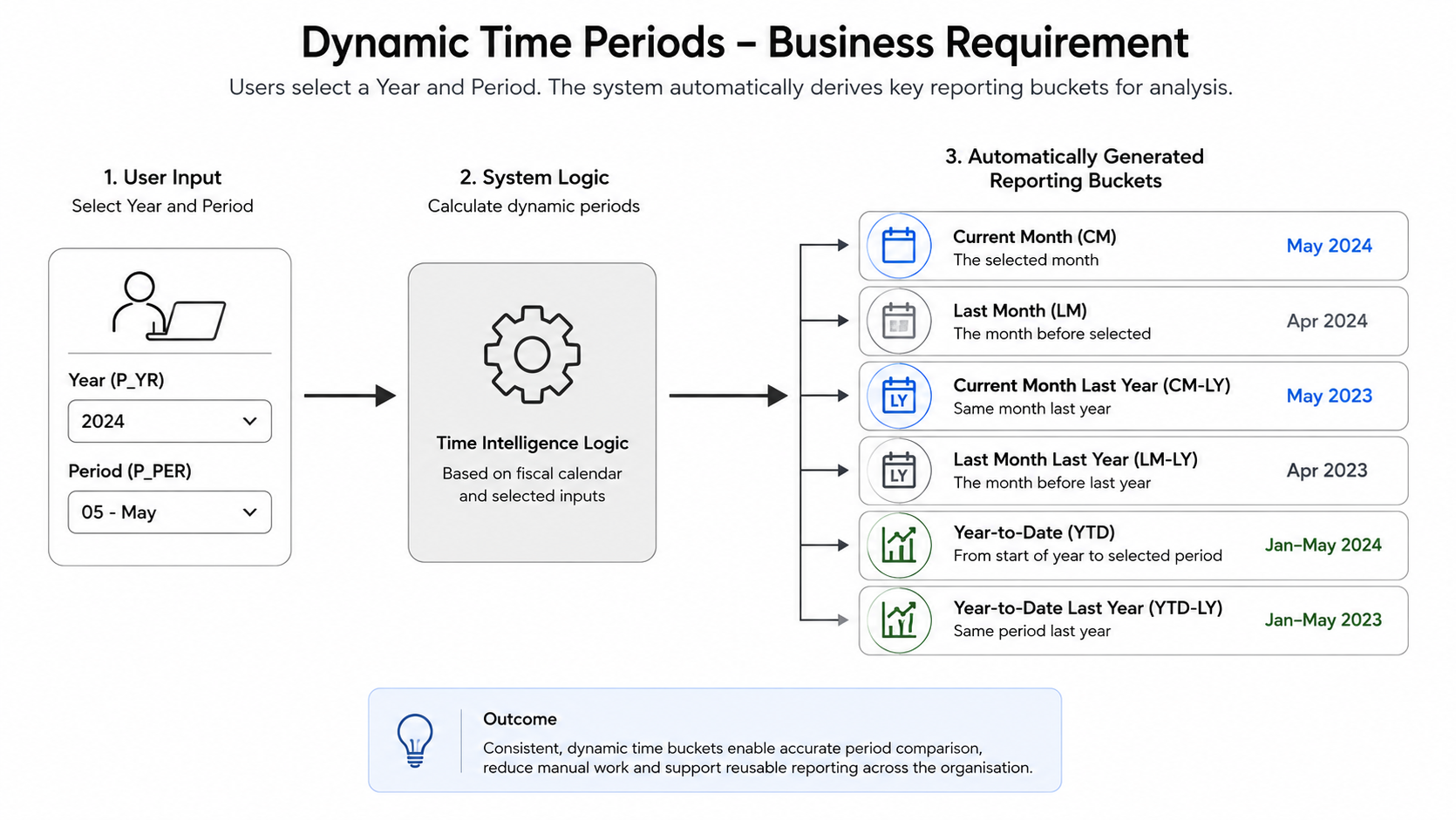
In almost every organisation, the same reporting requirement appears repeatedly: dynamic time periods.
Business users want to enter a date, month or fiscal period and have the analytics model automatically determine the reporting buckets that matter to them. Typical examples include:
- Current Month (CM)
- Last Month (LM)
- Current Month Last Year (CM-LY)
- Last Month Last Year (LM-LY)
- Year-to-Date (YTD)
- Year-to-Date Last Year (YTD-LY)
- Inception-to-Date (ITD)
The exact naming may vary by organisation, but the underlying requirement is consistent. A user selects a reporting period once, and the model derives all the related comparison periods automatically.
Without this capability, reports quickly become difficult to maintain. Developers may hard-code dates, create multiple versions of the same report, or push calculation logic into SAP Analytics Cloud stories. These approaches may work in the short term, but they are weak foundations for enterprise reporting.
Product limitation and roadmap context
In legacy SAP toolsets such as SAP BW and BW/4HANA, this requirement was often solved using variable exits. Variable exits allowed developers to use custom logic to derive additional selections from the user’s input before the query executed.
SAP Datasphere Analytic Models provide Input Parameters and Variables, but they do not currently provide the same variable-exit style scripting model that many BW teams are used to. Restricted Measures are powerful, but they should not be treated as a place to repeatedly rebuild complex date logic in every model.
SAP continues to expand Analytic Model capabilities. The roadmap has included areas such as variable derivation, calculation variables, multi-fact modelling, business layer support, additional calculation options and further BW-style analytical features.
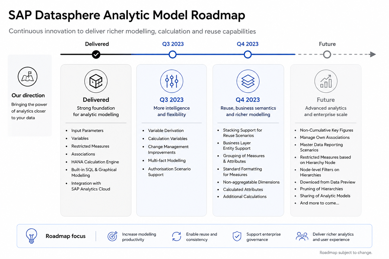
Those improvements are important, but the architectural question remains: where should dynamic time logic live so that it is maintainable, reusable and consistent across multiple reporting models?
Architecture overview
Black Barn recommends implementing dynamic time periods through a reusable Time Dimension.
The pattern is simple:
- The user selects a reporting year and reporting period.
- Input Parameters pass those values into the Time Dimension.
- The Time Dimension calculates reusable period flags.
- Analytical Datasets associate to the Time Dimension.
- Analytic Models create Restricted Measures using the calculated flags.
- SAP Analytics Cloud and other consumers receive consistent dynamic measures.
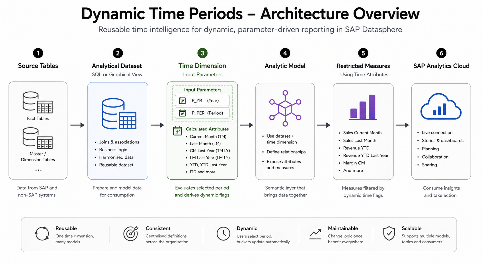
This design separates time intelligence from individual reporting models. Instead of copying the same logic into every Analytical Dataset, the logic is maintained once and reused wherever it is needed.
Input parameters
The solution normally starts with two simple Input Parameters:
| Parameter | Purpose |
|---|---|
P_YR | Selected reporting year |
P_PER | Selected fiscal or calendar period |
These parameters are supplied by the user and drive the dynamic calculations in the Time Dimension.
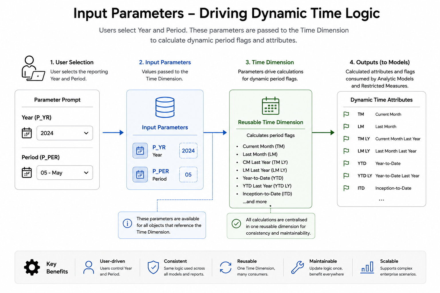
For fiscal calendars, the period format should be standardised and documented. For example, some models use fiscal periods such as 001 to 012, while others use calendar months. Mixing formats across models is one of the easiest ways to create inconsistent reporting.
Dynamic Time Dimension
The Time Dimension contains calculated attributes that determine whether each period belongs to a specific reporting bucket.
Typical calculated attributes include:
| Attribute | Meaning |
|---|---|
TM | This Month / Current Month |
LM | Last Month |
TMLY | This Month Last Year |
LMLY | Last Month Last Year |
YTD | Year-to-Date |
YTDLY | Year-to-Date Last Year |
ITD | Inception-to-Date |
Each attribute evaluates the selected year and period, then marks the matching rows with a simple flag such as X.
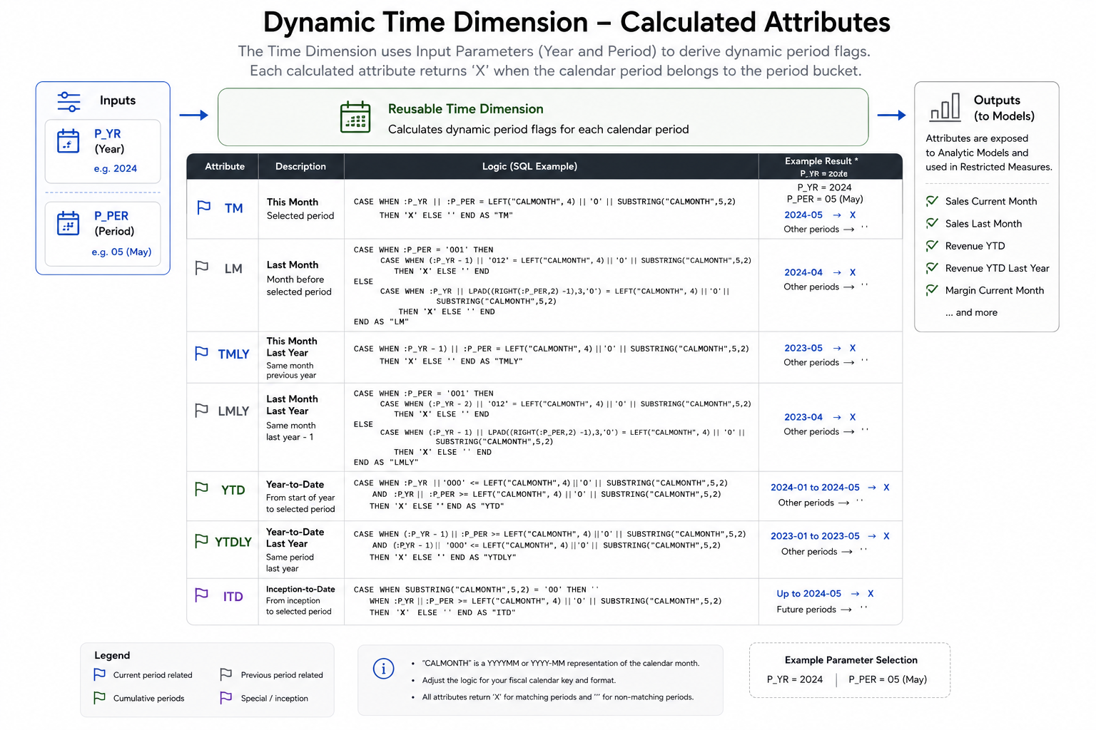
A simplified example of the pattern is shown below. The exact SQL should be adapted to the organisation’s fiscal calendar, period format and naming conventions.
CASE
  WHEN :P_YR || :P_PER = LEFT("CALMONTH", 4) || '0' || SUBSTRING("CALMONTH", 5, 2)
  THEN 'X'
  ELSE ''
END AS "TM"
More advanced expressions can then handle prior periods, year-end boundaries and year-to-date ranges. The important principle is that the complexity remains centralised in the Time Dimension rather than being repeated across every consuming model.
Restricted measures
Once the Time Dimension exposes calculated flags, the Analytic Model can use those flags to define Restricted Measures.
Examples include:
- Sales Current Month
- Sales Last Month
- Revenue YTD
- Revenue YTD Last Year
- Margin Current Month
- Margin Last Month
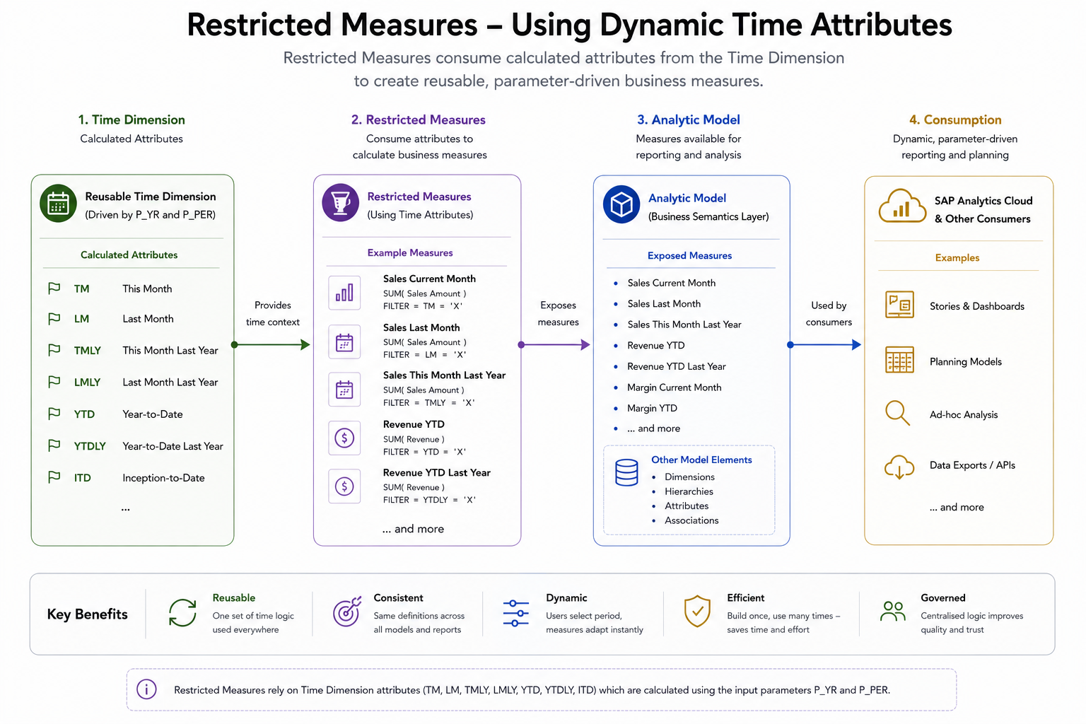
This keeps the reporting layer clean. The Restricted Measure does not need to understand how Last Month or YTD is calculated. It only needs to filter on the relevant flag from the associated Time Dimension.
Why reusability matters
It is technically possible to build dynamic time logic directly into an Analytical Dataset using either a SQL View or a Graphical View. For a single model, that may appear faster.
The problem appears later.
As more models are created, the same period logic is copied again and again. Any enhancement, correction or fiscal calendar change must then be applied repeatedly. This increases testing effort and introduces the risk that different reports define the same time bucket differently.
A reusable Time Dimension avoids that problem.
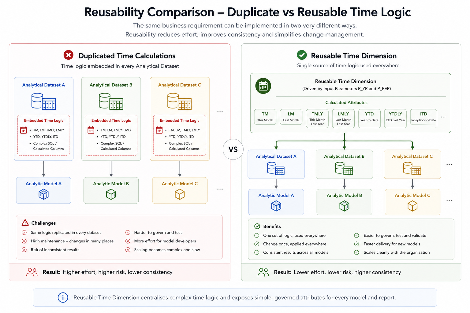
Centralising the logic provides clear benefits:
| Design choice | Impact |
|---|---|
| Time logic inside every Analytical Dataset | Fast for the first model, but difficult to govern and maintain. |
| Time logic inside SAP Analytics Cloud stories | Flexible for a single story, but weak for enterprise consistency. |
| Time logic inside a reusable Time Dimension | Strongest option for consistency, reuse, testing and long-term ownership. |
Step-by-step implementation pattern
A practical implementation usually follows this sequence.
1. Confirm the calendar basis
Decide whether the model uses calendar months, fiscal periods or a custom reporting calendar. Do not start with SQL until the business calendar has been confirmed.
2. Create or reuse the Time Dimension
The Time Dimension should contain the period keys required by the reporting models. For example, it may include calendar month, fiscal year, fiscal period, quarter, year and text attributes.
3. Add Input Parameters
Add parameters such as P_YR and P_PER. These values should represent the user’s selected reporting context.
4. Add calculated attributes
Create calculated attributes for the required time buckets. Start with the core requirements first: Current Month, Last Month, YTD and prior-year equivalents.
5. Associate the Time Dimension
Associate the Time Dimension to the relevant Analytical Dataset or fact model using the appropriate time key.
6. Create Restricted Measures
In the Analytic Model, define Restricted Measures using the calculated flags from the Time Dimension.
7. Test boundary conditions
Pay particular attention to period 001, year-end transitions, leap years if dates are involved, and fiscal calendars that do not align to the calendar year.
Best practices
Keep the model simple for consumers. Business users and report developers should see clean measure names such as Revenue YTD or Sales Last Month, not complex period derivation logic.
Use consistent naming. If one model uses YTDLY and another uses PYTD, the reporting estate becomes harder to understand. Establish the naming convention once and use it everywhere.
Avoid unnecessary time buckets. It is tempting to create every possible comparison period, but each one adds maintenance and testing effort. Build what the business actually needs.
Document the calculation rules. The Time Dimension should be easy for another developer to understand. Comments in SQL Views and clear business descriptions are valuable.
Common mistakes
The most common mistake is duplicating the same time logic across multiple models. This creates inconsistent definitions and makes future changes more expensive.
Other common issues include:
- hard-coding reporting periods;
- mixing fiscal and calendar logic;
- calculating time buckets inside SAP Analytics Cloud when they should be governed centrally;
- failing to test January or period 001 scenarios;
- exposing too many technical attributes to business users;
- creating Restricted Measures that are difficult to trace back to business definitions.
Performance considerations
Dynamic time logic is usually not the largest performance driver in an SAP Datasphere model, but poor design can still create unnecessary complexity.
The Time Dimension should remain small, selective and easy to join. The calculated flags should evaluate against a compact set of period records, not against unnecessarily large transactional datasets.
Where possible, keep the fact model focused on measures and keys, and keep the period intelligence in the dimension layer. This improves readability and reduces the temptation to duplicate logic in multiple places.
Black Barn recommendation
Black Barn recommends treating dynamic time intelligence as shared business logic, not as report-specific logic.
For most SAP Datasphere implementations, the preferred pattern is:
- reusable Time Dimension;
- clear Input Parameters;
- calculated period flags;
- Restricted Measures in Analytic Models;
- consistent naming and testing across all consuming models.
Even as SAP continues to enhance variable derivation and Analytic Model capabilities, this pattern remains valuable because it centralises business definitions and reduces duplicated modelling effort.
Further reading
SAP documentation and community articles
- Fiscal calendar generation for SAP Datasphere using built-in procedure | SAP Blogs
- SAP Datasphere Analytic Model Series – Calculated and Restricted Measures | SAP Blogs
- SAP Datasphere Analytic Model Series – Using Variables in Analytic Model | SAP Blogs
- Passing Input Parameters from Analytic Dataset to Analytic Model in SAP Datasphere | SAP Blogs
Conclusion
Dynamic time periods are a foundational requirement for enterprise reporting. SAP Datasphere can support this requirement effectively, but the design needs to be deliberate.
A reusable Time Dimension driven by Input Parameters provides a clean and maintainable way to derive Current Month, Last Month, YTD and prior-year comparison periods. Restricted Measures can then consume those flags without duplicating calculation logic across every model.
The result is a more consistent reporting estate, lower maintenance effort and a better foundation for future SAP Datasphere and SAP Business Data Cloud development.
Black Barn provides architecture, implementation, training and advisory services for SAP Datasphere, SAP Analytics Cloud and SAP Databricks.